ECE 5725 Final Project: HoloTracker
Corson Chao and Jay Chand
cac468 and jpc342
Demonstration Video
Introduction
HoloTracker is a project involving computer vision and multiprocessing with a Raspberry Pi to track the movements of an athlete performing his or her sport within view of surrounding cameras. The person in view of the cameras can see themselves being shown in a holographic, color display that isolates their body and creates the illusion of being a 3D rendering of that person. The inspiration for this project is that it combines many of the things that the team, Corson Chao and Jay Chand, enjoys and finds interesting, from sports and computer vision to holograms. HoloTracker is what we came up with. It has a fairly large setup that is visualized in Figure 1. The base station consists of one Raspberry Pi that is connected through HDMI to an external monitor, on which we run the Raspberry Pi Desktop by running the startx command on the console. This monitor is used to display four images that each reflect of the four sides of our display, which is a reverse-pyramid-shaped structure of plastic sheets that the “hologram” can be seen on. The rest of the setup consists of three USB cameras that connect to the Raspberry Pi. The person can stand inside the view of these cameras and move around there. The fourth USB slot is used to connect a keyboard from which we can control the Raspberry Pi.
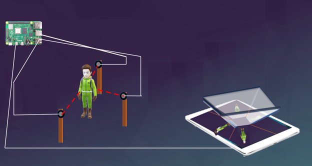
Figure 1: Overview of the project setup
Project Objective:
The goal of HoloTracker is to be able to holographically display the actions of a person through the use of a multi-camera setup. This project can ideally be used as a prototype for athletes to be able to perform their sport-relevant actions in view of the cameras (like running on a treadmill) and see their isolated and highlighted form in a display.
Design and Testing
Setup Details
For our end result set-up, in camera visualization, we used 2 Microdia (1920 x 1080) Cameras and 1 PlayStation Eye (640 x 480) camera. One of each camera is shown below in Figure 2.
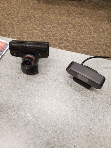
Figure 2: PlayStation Eye Camera on the left, Microdia to the right
For the placement of these cameras at the appropriate height and distance, we used three camera stands, and 5 USB extension cables. This set-up was then connected to a Raspberry Pi through the USB ports. This set-up is shown in Figure 2 below.
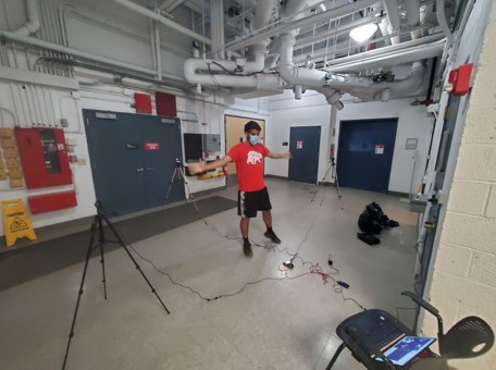
Figure 3: Our 3 camera set up connected to the Raspberry Pi, powered by the portable power source.
For the display portion, the Raspberry Pi was connected to a (11.5” x 14”) monitor through a micro-HDMI to HDMI connector. A plastic sheet cut into trapezoids was then placed on top of the display monitor for the hologram illusion. This part of the apparatus is shown below in Figure 4.
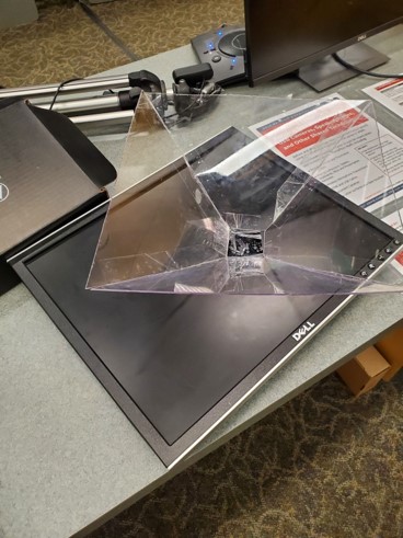
Figure 4: Orientation of the Hologram sheets on the Dell Monitor
The hologram sheets were oriented offset to the monitor due to the cutting of the display into being a 11.5” by 11.5” screen. Since the prism structure is square at the base, we used a square section of the screen as well. Also, since the model to be shown will be a person, we offset the display to being diagonal to the hologram so most height can be shown. More detail will be provided in the Holographic Displays section.
Camera Display
For the display of the two types of cameras shown in Figure 1, there were many adjustments that needed to be made, allowing cohesiveness and integration of the different types. OpenCV’s recording capabilities were used for the recording. The most simple change that needed to be done was to adjust the resolution of the two types of cameras to be of the same resolution. This needed to be done not as much due to the cohesiveness of appearance on the four faces, but rather more to allow similar processing speed of the images from all four cameras. If two of the cameras were at higher resolution than the other two, the processing speed would become slower, causing the display to be slowed down in real time and possibly causing the video to be showing different timeframes and lag times due to it. To check the resolution of each camera, we installed the v4l-utils package into linux, which allows the monitoring of different video outputs for linux devices. With this package we first checked the standard v4l-utils command, which showed the resolutions of each camera, showing the Microdia of 4 possible standard resolutions with the highest and standard being 1920 x 1080 while the max for the Play Station Eye’s being 640 x 480. As 640 x 480 resolution was also one of the Microdia outputs, we set that as the recording resolution for the four cameras before we began recording.
After the adjustments were made to OpenCV’s recording resolution, we used the cv2.VideoCapture(#).read()function to read the images within the video recording of the cameras. To successfully run the camera reading, the video output that the certain camera is registered as within the Raspberry Pi /dev needed to be found. To find this, we utilized the command v4l2-ctl -utils--devices from the previous v4l package. Tis command gave us the output below with the two Microdia cameras having 4 video outputs each for some reason while the Play Station Eye’s only had 1 each. While all cameras were just listed as USB camera, we found which one was which through constant plugging and unplugging. The output of this command is shown below:
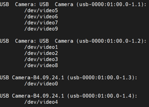
Figure 5: v4l2 output of camera output locations
Using an initial prototype function, we tested each of these /dev/video outputs to check if they all worked and we found that for the two Microdia cameras, only their first video output was functional while the other ones would not work and would cause errors. For example, for the second Microdia camera, using /dev/video1 in the read() function would allow video output, while 2,3, and 8 would just cause an error, leading to a video output error. With this error in mind, we planned on using only the main camera output of each camera, being in this case 0, 1, 4, and 5. With each time the RPi was rebooted though, the number order would change though, and each time the cameras were plugged and unplugged too quickly, the video outputs would go to even higher numbers like /dev18 or /dev19. These changes led to errors many times, especially when there is no /video0 output, which causes nothing to be run. We then learned to use v4l2-ctl --list-devices and change the video output location accordingly every time before running. With this method, we ran the video recording and combining successfully a couple times before it started to crash. After researching, it was found to be due to OpenCV being programmed to allow a maximum of 8 video outputs. So if the USB camera output switched to become /dev/video8 or higher, OpenCV would stop working.
Since this was the case, we tried to manually delete and change the video output order using sudo mv and sudo rm functions. Using sudo rm, we tried to delete and remove the video outputs of the Microdia cameras that were not useful, leaving only one output for each. We learned after a few tests that this ends up permanently affecting the RPi’s ability to read the camera output and sometimes corrupts the Pi. In the diagnosing of why the cameras were no longer compatible with the Pi, we had to reset and back-up the Pi a couple of times. In the end, we found the solution to this issue being to never delete the camera outputs but to keep moving them around. Every time the Pi is reset, it would be necessary to move any /dev/video outputs in the 0,1,2,and 3 positions to arbitrary far unused numbers like 17, 18, 19, and 20, while then moving the main video#’s of the four cameras to the 0, 1, 2, and 3 positions.
Another problem we faced with the cameras was sometimes it would try and start recording before the cameras were done setting up. This would also result in errors that caused the code to stagnate and not finish, and over time as we had to keep ctrl-C out of it, it seemed to affect the RPi interaction as well. To prevent this, we added a couple safety barriers to keep the camera from reading photos if the camera was not ready. One was to only run the reading and processing if cam.isOpened(), meaning the camera was ready to begin giving signal. We added another safety of taking the camera’s read output of ret that gives a True/False statement of whether an image was successfully output. If not, then the code is set to break out of the loop instead of attempting to process a non-existent image. This setting can lead to runs once in awhile not executing, but this is far preferable to the camera breaking. As another security precaution, we also added a waitkey, so if we wanted the code to stop halfway, we could press ‘q’ on the keyboard to break out of the loop.
Computer Vision
To get the desired output image, we applied a few stacked image processing methods. We tried multiple different high-level methods, which I will discuss later. The one we finally decided on was the following.
First, we applied Background Subtraction to the camera output. This is a module provided by OpenCV that is meant to find the “foreground” objects and pixels and get rid of the “background” objects and pixels. They have multiple different models for it, which use different already-trained methods, but the one that worked the best for us was the K-Nearest Neighbors (KNN) model. One other that we tried and worked somewhat well was MOG2, but we found it was not quite as accurate as the KNN model. The video background subtraction from OpenCV uses motion of some pixels and the locations of the pixels that stay “stationary” (keep relatively the same values within a certain threshold). This results in a binary image that separates foreground and background somewhat accurately, with some anomalous pixels from things like shadows and random movement in the background.
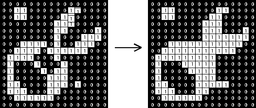
To get rid of some of those anomalous pixels, we used Median filtering with a kernel size of 9. This runs over each of the pixels in a frame from a camera and sets each pixel value to the median of the surrounding pixels (in our case, 4 pixels in every direction). This is a form of nonlinear low pass filtering that is less blurring than an averaging or Gaussian blurring filter. Median filters get rid of “salt and pepper” noise, or anomalous spots in the image. It smooths the image to where only the “main” or large objects in the binary image remain. An example of median filtering can be seen in Figure 6.
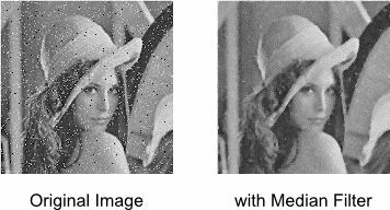
Figure 6: Example of the effects of median filtering on an image: getting rid of salt and pepper noise
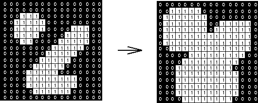
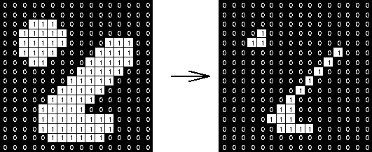
The final filter we applied on this now-binary image was Morphological Closing in order to partly fill in gaps in objects. This is a combination of two other Morphological processes: Dilation followed by Erosion. The term “morphological” in image processing refers to filters or operations on an image that are based on the shapes of objects in the image rather than just individual pixel values. In order to do this, morphological filtering algorithms typically involve checking each pixel’s neighbors’ values and acting accordingly. In binary images, neighboring pixels of the same value are seen as connected and can be seen as part of an “object.” The process of Dilation involves adding pixels around the pixels that are considered the “edge” of an object (makes the outline of the object thicker), which makes objects bigger. Erosion is the opposite of this process, removing pixels from the edges of objects, which moves the edges of objects inward. Running these in succession means that first with Dilation, pixels are added both inwards and outwards to the edges, and then with erosion, the pixels on the outside are subtracted, which results in pixels being added to the inside of the object. This ultimately means gaps within images are filled. All of this can be seen in visual form in Figure 7.
(a)
(b)
(c)
Figure 7: Visualizations of morphological dilation, erosion, and closing, respectively.
In (a), dilation is shown, as pixels are added around the edges of the white object.
In (b) erosion is shown, as the opposite happens and every edge pixel (pixels that are not completely surrounded by white pixels) are removed.
Finally in (c), closing is shown, which is running dilation and then erosion on the input image shown.
Too much closing creates squares in the image that make everything look blocky and unrealistic. It also sometimes closes gaps that should not be closed, which can ruin the shape of the person in the image. Adjusting the “amount” of closing involves changing the kernel size, which just means adjusting how many pixels are added in dilation and removed in erosion. These operations stacked on top of each other result in creating an image that isolates a person from a camera’s video output, shown in Figure 8.
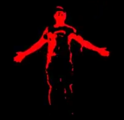
Figure 8: One example of a final image after our image processing. It shows the moving parts of the person and in a video format, looks quite realistic
Before settling on this method, we tried a few other things first, which did not work out nearly as well. The first attempt was to use Machine Learning-based human detection, trained and provided by OpenCV, to find the person in each camera’s video output. This allowed us to find the bounding rectangle around a person and create the ideal crop of the image to isolate a person. We would then use a median filter on this cropped image and then use edge detection to create an outline of a person. There were many problems with this, however, the first being that it was incredibly slow. The human detection took a long time and made it impossible to do anything even close to real time. It also was not always accurate, which led to a noticeable number of output frames that do not have a person included at all. The last problem with this method was that if we always crop the image to only include the person, the person would always be at the center of the display, which would be perfect for the ideal scenario where we would use a treadmill with an athlete; however, for our project, we were just trying to capture the movements of a person standing in the middle, and we wanted to include the motion within the frame in our display, so we did not want to crop the image at all.
The second method was a somewhat watered-down version of this, where instead of using human detection, we would try to use object tracking, which instead of detecting humans, would track an object whose starting point we would tell it as an input. It would ideally treat the person like just a connected set of pixels that it tracked to serve the same purpose as human detection but much faster. While this was faster than human detection, it was rarely accurate, as the image crops it created would consistently cut off part of the person’s face or just not get the person at all. When this did not work, we switched to the final method that was detailed above and that works far better and faster than either of these methods.
Multiprocessing
When we first performed the recording and merging on a single core, the extreme processing on a single core caused the video to become extremely lagged with real-time processing being impossible. Adding on the machine learning of the computer vision component, frames would be displayed so slowly that movements would not look cohesive and the machine learning algorithm would not have enough frames and precise enough movements to properly isolate the person. Due to these constraints, we used multiprocessing to allow all four cores to be utilized in the recording, processing, and merging of all the camera outputs. This change to multiprocessing allowed us to perform our display in real time without significant lag at around 5-8 fps.
In terms of allocation of core resources for the completion of the processing, our division of processes was to create two functions: camera and mergeall. The function camera performs the recording and image processing described above while mergeall would combine the images received into a single series of images (to make a video) in the correct orientation around the screen.
Multiprocessing was performed on the raspberry pi through the multiprocessing package. This package allows the separation of different functions into being performed and split amongst different cores.
To run the multiprocessing package we imported the multiprocessing Queue and multiprocessing Process for this purpose. These two packages allowed the functions to be run and for the memory to be stored and shared amongst the cores. In typical process running, the variable values would be stored in the local cache of a certain core since everything within the process would be done within the same core. If this assumption is used in multiprocessing, the variables even if made global would be unable to transfer to the other functions, which we learned through a lot of trial and error. So in the case of multiprocessing, we had to account for the fact that the process is split into different functions to be run by different cores. In this case, the memory to be shared would need to be stored in a shared memory location so the different functions can access it. For multiprocessing, this location is in the multiprocessing Queue.
In the initial stage, we thought that global variables that would not be changed throughout the process would also need to be independently loaded in each core, so we had all the variables loaded into the different functions. This slowed down the processes significantly, but then we found that unchanging variables could be stored outside of the functions and shared between all the cores. The variables that needed to be placed inside the queues instead were variables that would be changed in value throughout the process run. In our case, this was the images to be processed and displayed. The plan was to have the camera function run for each of the four camera outputs, and then store their processed images into the queue.
How the queue worked was that each time an image was pushed into the queue, it would add to the back of the memory stack within the queue, and each time the memory is accessed, or ‘popped’, it would take that piece of memory out of the stack from the front of the queue. And as these images are pushed into the queue, the mergeall function would pop the images out of the queue to merge them together. In our initial test, we had four camera outputs, and a single queue for the four outputs to store the images to be merged. The thought process was that as each of the cameras were in the same resolution with the same exact commands, they would keep running in the same order, so popping out of the queue into the merging function would always be in the same order. What we found through print functions was that the order of the four cameras pushing images into the queue would change in order. The small differences in the push order was due to the machine learning algorithm. With different directions having different difficulties of object isolation, the algorithm would take slightly longer or shorter in completing the processing step.
To solve this problem, we created four different queues instead, one for each of the four camera outputs. As four cameras were originally used, we created four separate queues for each of the cameras to send their images into for eventually sending to the mergeall function for merging. The order of events for the forming and executing of these queues was to first create the queues within an intro function called if __name__=='__main__' which would run before the main function. After the four queues were created, they would all be input into the main function as argument inputs as shown below:
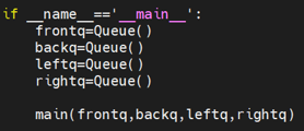
Figure 9: Multiprocessing Queue Creation
After the queues were placed into the main function, they were split into the independent functions each of them were to be modified by. Here is the point that the multiprocessing Process package was used. Each of the functions to be run was placed within the command of multiprocessing.Process(), which would place the functions within the parenthesis into different cores to be run. The functions to be run were four times of the camera function for each of the four cameras and once of mergeall to merge and display them. For the running of these five functions of four cores, our worry was whether the four cores could only run four functions at once, limiting our ability to run real-time, frame by frame. What we found though was that the multiprocessing function automatically splits processing time between functions throughout the cores.
As each camera function for each camera would only need to access the queue for its independent images, their only argument inputs were the camera video output number (/dev/video#), and its queue. These camera functions would keep pushing their images into their queue in this manner as the function was made to push the images taken and processed into the given queue. The mergeall function would then take all four queues as argument inputs and orient them accordingly for merging and outputting. After these functions were all created, they would all be run at around the same time using the start() function of the microprocessing package. This main procedure is shown below in Figure 10:
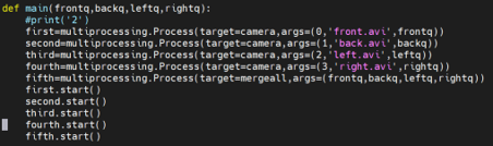
Figure 10: Creation of the multiprocessing functions
The ‘avi’ text inputs shown in purple above are unnecessary in the current running of the real-time code. We allowed the inputs of avi names in case the user wanted to perform video saving as well as real-time display. With the current speed of the processors with only four cores though, the user will have to choose between either displaying the outputs in real time or saving the videos. If both are attempted at the same time, the frames per second decreases to about 2 fps, drastically decreasing the “feel” of it being a video and also decreasing the capability and accuracy of the machine learning algorithm.
While we found that the multiprocessing worked with the five functions running at once, we found the processing rate to be much slower in speed. Using htop, we saw that all four cores were running at 100% capacity, sometimes even writing higher due to possible glitching and overloading. To decrease the glitching and to free up the cores slightly, we took off the right camera output, and instead just flipped the left camera output to create the right side image.
The updated procedure with this approach became having 3 cores process 3 camera outputs, and 1 core to take the 3 camera outputs, duplicate and flip the left output, and display the now four outputs.
Holographic Merging and Display
The holographic display component, shown in Figure 11, of our project consists of the external HDMI monitor connected to the Raspberry Pi, as well as plastic sheets that were cut and arranged into the shape of a reverse pyramid, with a small square base that opens up to have four, somewhat triangular side panes. These panes each show one viewing angle of the person moving in view of the cameras by reflecting the four images displayed on the monitor.
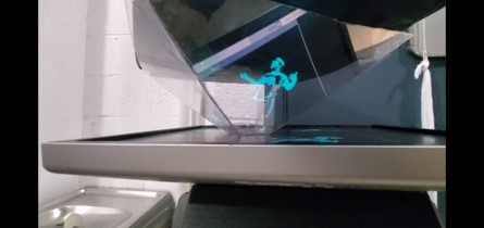
Figure 11: Screenshot from our video showing the holographic display showing a person
The images displayed are the ones that are returned from our computer vision methods. However, we only had three cameras and four panes to display. Using four cameras, as discussed elsewhere, was too much on the Raspberry Pi when we also had to merge the pictures onto a single display, and that is why we had three. To account for this, since our display really comes from 2D binary images on the monitor, we just flipped the image output from the “side” camera (while the other two were “front” and “back”) horizontally to show an image on the fourth side that matches up with the rest of the panes.
In order to merge the images, we used numpy’s stacking functions. Since the resulting merged image should have the front and back image be diagonal as well as between the left and right, the images, we stacked the front image on top of the left, and right on top of the bottom using vstack and then merged these two stacks together horizontally using hstack. To allow these four images to stack correctly and oriented all facing the center for the hologram placement, they were first all made into squares so that the stacking would create a square of the correct dimensions, and then they were all rotated around their centers, so that they will all face the center. After being merged correctly, the created image was scaled up appropriately to the size of the computer screen as necessary to a 1000 x 1000 pixel square.
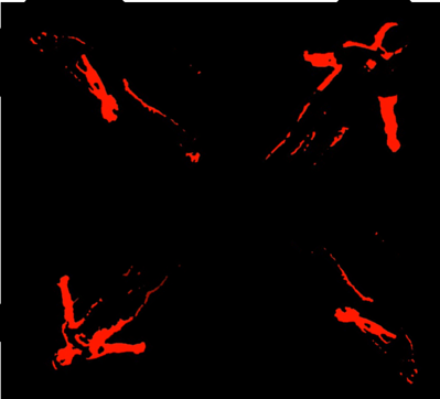
Figure 12: Primitive Version of our merged processed Display
In this code as well, we added a couple of safety functions to allow proper execution of the code. Similarly to the camera code, there was a waitkey installed so that if the letter ‘q’ was clicked, the code would break out of the loop and exit. Another safety was that before the code began taking images out of the queue, it would check whether there is an image within the queue to process and take out. If not, it would wait until there is. This was done through importing the Empty package of the regular Queue package. It gives a True/False when used to check if the current queue is empty.
We also considered a potential issue of the image stretching when displayed on the plastic. This would happen because the surface that the image is projected onto is longer than the surface it comes from, so the light from the image (and therefore the image itself) would appear stretched, visualized in Figure 13.
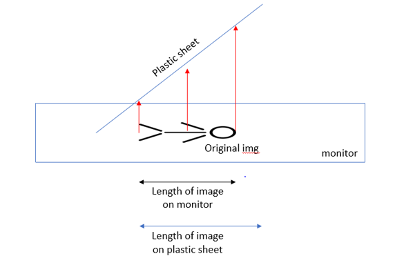
Figure 13: Stretching of image caused by projection, showing horizontal view of one plastic sheet
However, we realized that we did not have to worry about this for two reasons. First, the severity of this problem is proportional to the size of the setup. The bigger the image, the more pixels there are to stretch, and the bigger the plastic sheets, the greater the difference in length between the horizontal image and the reflected image. Second, this problem only exists if the image is viewed from an angle perpendicular to the plastic sheet pane; each pane is at a 45° angle to the monitor, which means when viewed from a horizontal angle, the “virtual image” from the reflection of the image is the exact same size as the original image. This is why the ideal viewing angle is horizontally into the pyramid, where displayed is a perfectly-sized virtual image whose “virtual origin” (or perceived origin) is the center of the pyramid, visualized in the ray diagram in Figure 14.
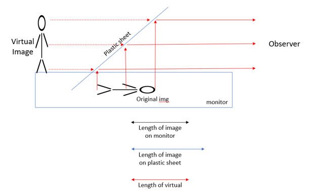
Figure 14: Ray diagram showing the virtual image effect of the hologram pyramid
While working on this part of the project, besides general issues with trying to make code that does what we want, the main problem we ran into was that part of the way through, our monitor just stopped working. It was clear that it could be detected and there was some signal between our Raspberry Pi and the monitor, but for some reason, it would not display anything after previously being able to display an extension of one of our laptops as well as the Raspberry Pi. We tried different cables and different adapters that could plug into the Raspberry Pi, but none of that worked, so we decided to take the monitor in to Professor Skovira, who checked the monitor with his own Raspberry Pi and helped us realize the monitor must have just stopped working on its own. This problem forced us to delay our final demo by one day so that we could reintegrate a new working monitor into our project, which we were able to do, so we ended up with a working hologram display.
The hologram is not perfect, however, for three main reasons. First, the display pyramid has corners, which do not provide a smooth transition point between two different panes but instead serve the purpose of providing a boundary between the panes where the virtual images do create the illusion of a 3D holographic rendering in the center of the pyramid. The second reason is that the cameras were very difficult to get perfectly aligned. In order to create the most believable illusion possible, the cameras must be aligned such that the motion of each side matches up perfectly with the others, and this was extremely difficult to make happen. Ideally, whoever might use this would be using an already-calibrated setup that is perfectly aligned to capture the person’s movement on a stationary treadmill or something similar, in which case this would not be a problem. Finally, the third main issue with the display is the lag resulting from the large CPU usage on the Raspberry Pi. Not only does this force us to have a slow frame rate with between 0.5 and 1 second delay between the person moving and the display updating, but it also causes each pane’s updates to happen at slightly different times, so the angles of movement do not perfectly match up. A viewer can tell that they are representing the same actions, but ideally, these would be perfectly in sync with each other and faster to create a convincing and smooth hologram. One solution to this problem would be to use multiple Raspberry Pis so that each could focus on one or two cameras, which method would involve a lot more integration work but would work to increase the efficacy of HoloTracker.
Results and Conclusions
The end result of the work detailed above was a fully functional setup that displayed the actions of a person who moved in the space between the cameras as a holographic display.
Overall, this lab was a great success in which we gained valuable experience and learned a lot, while also coming out of it with a very interesting end product. The troubles we had with hardware like cameras and the monitor not working properly as well as the issues that came from doing the project itself taught us a lot about integration and gave us experience that will help us improve our approach to doing these things in the future. Hopefully, the things we learned through this experience will also be able to help future students who try anything similar because they will know about the problems we faced beforehand and be better prepared to deal with them.
Some of the main things we learned about while doing the project were computer vision, multithreading, and integration of a full system. In trying to extract exactly the image we wanted for our display, the multiple different methods we employed taught us about how various computer vision and image processing operations work in different environments and on different images/videos. Then, while trying to merge the outputs of the three cameras, we gained experience in trying to work with Linux to take advantage of the structure of the Raspberry Pi and its ARM processor to optimally use the CPU and get the desired output. Specifically in this area, we learned how to make shared queues between the processors and use them to make sure our overarching merging function can access all the data it needs to. Overall, the many lessons in engineering and in troubleshooting problems will absolutely help us in the future when we try to implement and integrate any full system.
Future Work
The end result of the work detailed above was a fully functional setup that displayed the actions of a person who moved in the space between the cameras as a holographic display. There are a few things we have thought of that would further this project to a point of greater usability or effectiveness. The first one relates to one of the first problems we had with the cameras, which is that two of the cameras were assigned to four inputs each. A potential solution to this would be to use the same type of camera in all locations, and ideally cameras that do not get assigned to four inputs each. In the case that they are assigned to multiple inputs, it would be beneficial to find a way to automatically extract the one correct input from each so that the user does not have to manually change them around.
Another addition that fits naturally into our goal for the project would be to add a treadmill into the viewing area of the cameras and stable stands for the cameras to have a perfect view of the person on the treadmill. This would bring the project closer to a case where it can actually be usable, once the framerate and lag is improved.
In order to improve these things, one possible method would be to use two Raspberry Pis instead of one and integrate them such that their timing is synchronized. This would allow us to use four cameras instead of just three for a truly full view of the person, and it would also allow us to use the machine learning and computer vision methods that were too slow earlier because of increased computing power. One other benefit of this is that with increased memory from multiple Pis, we could save the videos we create as well as display them live. This would be greatly beneficial but also more costly, so this would be a much larger scale project.
Another potential addition to HoloTracker would be to use servo motors to move or rotate the cameras to change or keep the view of a person as the person moves, allowing a real 360 view. This could be done by using human detection from OpenCV with multiple Raspberry Pis to center the view on the person or move it to another desired location.
One other small addition to the project would be to create a PyGame interface where the user can run and re-run the program once it finishes so that we would not have to use a keyboard in the console to run the program.
Budget
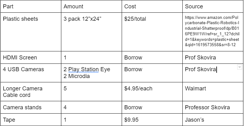
Parts List and Budget
Work Distribution
For the development of this project, we started off with working together to figure out how to get video output from the camera and how to record videos of a specified resolution. To make prototyping code easier, we started off with using recorded video rather than live streaming. Corson recorded his friend doing different actions in front of a camera with different angles, and we used this video to create into frames for the machine learning and merging video components. It was after we completed these parts that we began attempting live-streaming.
For the following work, Jay was in charge of the video processing component while Corson worked on the video merging and multiprocessing components. After completing these components, we merged these together and worked on assembling the hardware components together.
Team Photos
Corson Chao (cac468)

Jay Chand (jpc342)
References
DIY Hologram SetupCanvas References
Detecting HDMI Monitors Forum
More HDMI References
Startx over SSH
Displaying Connected Displays
OpenCV Reference
Multiprocessing
Multiprocessing Queues
Communication Between Processes
More on Multiprocessing Queues
Image Collages
Morphological Image Processing
Minimum, Maximum, and Median Filters
Setting VidCap Resolution
Code Appendix
import cv2 #for image processing
import numpy as np #for image stacking
import time #
import matplotlib.pyplot as plt
import multiprocessing
from Queue import Empty
from multiprocessing import Process, Queue
import random
med_val = 9 #medium value for grainy filtering
edge_1 = 70 #high threshold for intensity gradient
edge_2 = 70 #low threshold for intensity gradient
size=3 #size of shape, side length
fps=8 #frames per second, checked experimentally through recording
length=80 #number of seconds to run
kernel=np.ones((size,size),np.uint8) #set size of shapes to fill in for
set_color=[random.randint(0,255), random.randint(0,255), random.randint(0,255)]
#make the color of the display keep changing just to look cool
loops=fps*length #sets the amount of loops for frames to be run
#print('1')
#frontf=cv2.imread('/home/pi/Lab5/background.png',cv2.COLOR_RGB2GRAY)
#leftf=frontf
#rightf=frontf
#backf=frontf
#print('start')
def camera(dev,name,queue): #function that takes in the video /dev/video# number, name of video if desired to be saved, and the queue to save within
cam=cv2.VideoCapture(dev)
cam.set(3,640) #set the width of the recording from the camera as 640 px
cam.set(4,480) #set the height of the recording from the camera as 480 px
fg1=cv2.createBackgroundSubtractorKNN() #function to apply background subtractor on pic
#fourcc =cv2.VideoWriter_fourcc(*'XVID') uncomment to record video
#out=cv2.VideoWriter(name,fourcc,fps, (480,640)) uncomment to record
loopnum=0 #number of loops for changing frames the code has gone through
while(loopnum<loops and cam.isOpened()): #if recording not over and cam is ready
ret, frame=cam.read() #check the ret (whether has pic) and frame (pic)
if not ret: #if a picture wasn't taken)
print("not ret") #say not ready
break #break out of loop so it doesn't have an error
#filtering for object detection
write=fg1.apply(frame) #apply the background subtractor on pic
write=cv2.rotate(write, cv2.ROTATE_90_CLOCKWISE) #rotate since the cameras are sideways to record longways
write = cv2.medianBlur(write,med_val) # Median filter for grainyness
write = cv2.Canny(write, edge_1, edge_2) # Edge detection
write=cv2.morphologyEx(write,cv2.MORPH_CLOSE,kernel) #closes insides of shapes to be cohesive
write = cv2.cvtColor(write, cv2.COLOR_GRAY2RGB) # Convert to color format so that the writing works
write[np.where((write!=[0,0,0]).all(axis=2))]=set_color #change the binary foreground made by machine learning into the chosen color
# Write out to new file
#out.write(write.astype('uint8'))
queue.put(write) #put the processed image into the present queue
# Live display
#cv2.imshow('frame', write) # Should be changed to be the display code for the hologram display, shows the one camera processed
# Breaks the loop if the user types q
if cv2.waitKey(1) & 0xFF == ord('q'):
break
#cv2.imshow('backf',backf)
loopnum = loopnum + 1 # Increment loop (frame) counter
# Release inputs and outputs and close any extra windows
cam.release()
#out.release()
cv2.destroyAllWindows()
print('Done')
#running=False
def mergeall(frontq,backq,leftq): #takes the queues as input from front, back, and left cameras to merge into a single photo/video
#(h,w)=backf.shape[:2]
h=640 #gives the current height of frame, now tall after rotate
w=480 #gives current width, shorter since rotate
center=(w/2,h/2) #gives center of picture to rotate around
while not leftq.empty(): #left queue should be last to fill, so if it is still empty, wait until it has something to start merging
print('waiting for camera input')
while True: #only breaks when the queues become empty
frame1=cv2.resize(frontq.get(), (480,480)) #crop the image to square
frame2=cv2.resize(backq.get(), (480,480))
frame3=cv2.resize(leftq.get(), (480,480))
frame4=frame3 #make the right image same as the left
#if frontq
M1=cv2.getRotationMatrix2D(center,315,1.0) #make the necessary rotations for the display around the center of each
frame1=cv2.warpAffine(frame1,M1,(w,h))
M2=cv2.getRotationMatrix2D(center,315,1.0)
frame2=cv2.warpAffine(frame2,M2,(w,h))
M3=cv2.getRotationMatrix2D(center,225,1.0)
frame3=cv2.warpAffine(frame3,M3,(w,h))
M4=cv2.getRotationMatrix2D(center,45,1.0)
frame4=cv2.warpAffine(frame4,M4,(w,h))
col1=np.vstack([frame1,frame3]) #stack the top and right frame
col2=np.vstack([frame4,frame2]) #stack the left and bottom frame
#cv2.imshow('dst',dst)
collage=np.hstack([col1,col2]) #combine the two stacks to make 2x2
collage=cv2.resize(collage, (1000,1000)) #increase size to match screen
#display=':0.1.1388' #attempt at ssh onto a hdmi screen
#os.environ['DISPLAY']=display
#print(os.environ['DISPLAY'])
#cv2.imshow('window on %s'%display,collage)
cv2.imshow('collage',collage) #display the collage onto screen
#fourcc =cv2.VideoWriter_fourcc(*'XVID')
#out=cv2.VideoWriter('store.avi',fourcc,5, (600,600))
#out.write(collage)
key=cv2.waitKey(1) #deleted the waitkey to make it just end when the queues empty out
#print('merge')
if frontq.empty() and frontq.empty() and leftq.empty(): #end when the queues empty and cameras stop recording
break
cv2.destroyAllWindows() #clear windows
def main(frontq,backq,leftq): #main function to execute the side functions
#print('2')
#makes each function go in as a multiprocessing process with the arguments of the camera video input, the desired avi name if to be saved, and the queue to input into
front=multiprocessing.Process(target=camera,args=(0,'front.avi',frontq))
back=multiprocessing.Process(target=camera,args=(1,'back.avi',backq))
left=multiprocessing.Process(target=camera,args=(2,'left.avi',leftq))
#right=multiprocessing.Process(target=camera,args=(3,'right.avi',rightq))
combine=multiprocessing.Process(target=mergeall,args=(frontq,backq,leftq))
front.start() #start the functions
back.start()
left.start()
#right.start()
merge.start()
if __name__=='__main__': #creates the queues and inputs them into the main
frontq=Queue()
backq=Queue()
leftq=Queue()
#rightq=Queue()
main(frontq,backq,leftq)
#print('3')